Overview

The configuration interface allows for high-performance training and evaluation of models without need for writing code.

Configuration files are defined in YAML format and are grouped up into four sections:

Model: Defines the architecture of the model, neighbor sampling configuration, loss, and optimizer(s)
Storage: Specifies the input dataset and how to store the graph, features, and embeddings.
Training: Sets options for the training procedure and hyperparameters. E.g. batch size, negative sampling.
Evaluation: Sets options for the evaluation procedure (if any). The options here are similar to those in the training section.

Link Prediction Example

In this example, we show how to define a configuration file for training a 3-layer GraphSage GNN for link prediction on fb15k_237.

This example assumes that marius has been installed with pip the dataset has been preprocessed with the following command:

marius_preprocess --dataset fb15k_237 --output_dir /home/data/datasets/fb15k_237/

1. Define the model:

model:
  encoder:
    train_neighbor_sampling:
      - type: ALL
      - type: ALL
      - type: ALL
    layers:
      - - type: EMBEDDING
          output_dim: 50
          bias: true

        - type: FEATURE
          output_dim: 50
          bias: true

      - - type: REDUCTION
          input_dim: 100
          output_dim: 50
          bias: true
          options:
            type: LINEAR

      - - type: GNN
          options:
          type: GRAPH_SAGE
          aggregator: MEAN
          input_dim: 50
          output_dim: 50
          bias: true
          init:
            type: GLOROT_NORMAL

      - - type: GNN
          options:
          type: GRAPH_SAGE
          aggregator: MEAN
          input_dim: 50
          output_dim: 50
          bias: true
          init:
            type: GLOROT_NORMAL

      - - type: GNN
          options:
          type: GRAPH_SAGE
          aggregator: MEAN
          input_dim: 50
          output_dim: 50
          bias: true
          init:
            type: GLOROT_NORMAL

  decoder:
    type: DISTMULT
  loss:
    type: SOFTMAX_CE
    options:
      reduction: SUM
  dense_optimizer:
    type: ADAM
    options:
      learning_rate: 0.01
  sparse_optimizer:
    type: ADAGRAD
    options:
      learning_rate: 0.1

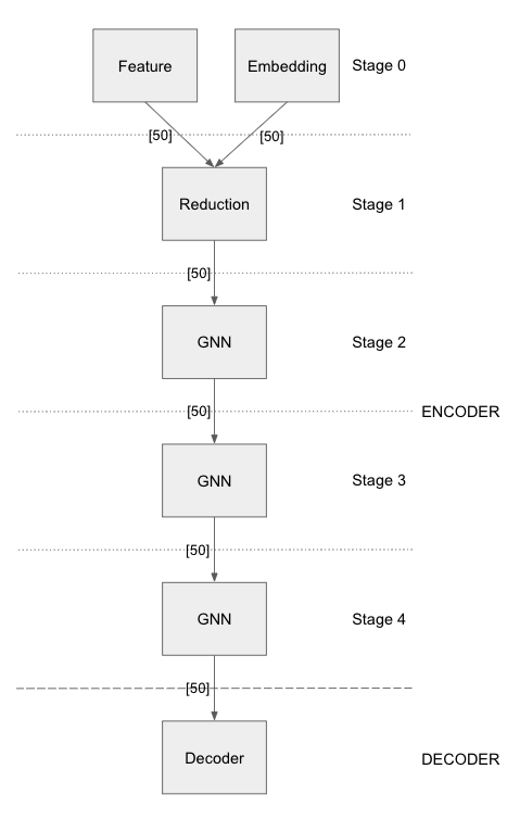
The above model configuration has 5 stages in the encoder section, each stage separated by a –. The first stage has 2 layers, one embedding layer with output dimension 50 and another feature layer with output dimension of 50. The reduction layer in stage 2 takes input the combined vector of dimension 100 and outputs a 50 dimensional vector. It is followed by 3 stages of GNN layers. The output from the encoder is fed to the decoder of type DISMULT. The loss function being used is SoftmaxCrossEntropy with sum as the reduction method. The dense optimizer is for all model parameters except the node embeddings. Node embedings are optimized by the sparse optimizer.

2. Set storage and dataset:

storage:
  device_type: cpu
  dataset:
    dataset_dir: /home/data/datasets/fb15k_237/
  edges:
    type: DEVICE_MEMORY
    options:
      dtype: int
  embeddings:
    type: DEVICE_MEMORY
    options:
      dtype: float

The storage configuration provides information on the location and statistics of the pre-processed dataset. It also specfies where to store the embeddings and edges during training. The device_type is set to cpu here, cuda mode can be used for gpu training. DEVICE_MEMORY in this case states that the embeddings need to stored in cpu memory.

3. Configure training and evaluation

training:
  batch_size: 1000
  negative_sampling:
    num_chunks: 10
    negatives_per_positive: 10
    degree_fraction: 0
    filtered: false
  num_epochs: 10
  pipeline:
    sync: true
  epochs_per_shuffle: 1
  logs_per_epoch: 10
evaluation:
  batch_size: 1000
  negative_sampling:
    filtered: true
  epochs_per_eval: 1
  pipeline:
    sync: true

The training configuration specifies number of data samples in each batch and the total number of epochs to train the model for. Marius groups edges into chunks and reuses negative samples within the chunk. num_chunks`*`negatives_per_positive negative edges are sampled for each positive edge. Marius also uses pipelining to overlap data movement with training which introduces bounded staleness in the system. We can explicitly set sync to true if we want every minibatch to see the latest embeddings.

Node Classification Example

In this example, we show how to define a configuration file for training a 3-layer GAT GNN for node classification on ogbn_arxiv.

This example assumes that marius has been installed with pip the dataset has been preprocessed with the following command:

marius_preprocess --dataset ogbn_arxiv --output_dir /home/data/datasets/ogbn_arxiv/

1. Define the model:

model:
  learning_task: NODE_CLASSIFICATION
  encoder:
    train_neighbor_sampling:
      - type: ALL
    layers:
      - - type: FEATURE
          output_dim: 128
          bias: false
          init:
            type: GLOROT_NORMAL
      - - type: GNN
          options:
            type: GRAPH_SAGE
            aggregator: MEAN
          input_dim: 128
          output_dim: 40
          bias: true
          init:
            type: GLOROT_NORMAL
  decoder:
    type: NODE
  loss:
    type: CROSS_ENTROPY
    options:
      reduction: SUM
  dense_optimizer:
    type: ADAM
    options:
      learning_rate: 0.01
  sparse_optimizer:
    type: ADAGRAD
    options:
      learning_rate: 0.1

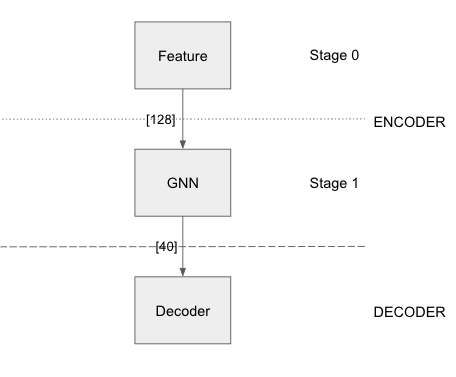
The above node classification example has 2 layers in the encoder section, one feature layer and another GNN layer. The number of training/evaluation sampling layers should be equal to the number of GNN stages in the model. The model has a decoder of type node classification. The loss function being used is Cross Entropy with sum as the reduction method.

2. Set storage and dataset:

storage:
  device_type: cuda
  dataset:
    dataset_dir: /home/data/datasets/ogbn_arxiv/
  edges:
    type: DEVICE_MEMORY
  nodes:
    type: DEVICE_MEMORY
  features:
    type: DEVICE_MEMORY
  embeddings:
    type: DEVICE_MEMORY
    options:
      dtype: float
  prefetch: true
  shuffle_input: true
  full_graph_evaluation: true

The storage configuration here is very similar to the one shown above in Link Prediction.

3. Configure training and evaluation

training:
  batch_size: 1000
  num_epochs: 5
  pipeline:
    sync: true
  epochs_per_shuffle: 1
  logs_per_epoch: 1
evaluation:
  batch_size: 1000
  pipeline:
    sync: true
  epochs_per_eval: 1

The above training configuration has specifications for a training batch size of 1000 and total epochs of 5. The logs_per_epoch attribute sets how often to report progres during training. epochs_per_eval sets how often to evaluate the model.

Defining Encoder Architectures

The interface enables users to define complex model architectures. The layers field can be seen as a double-list, a list of stages wherein each stage is again a list of layers. We need to ensure that the total output dimension of a stage is equal to the net input dimension of the next stage. We need to ensure that the following conditions are met while stacking layers of a model,

Embedding/Feature layers have only output dimension. The input_dim is set to -1 by default
A Reduction layer can have inputs from multiple layers in the previous stage and has a single output
The number of training/evaluation sampling layers should be equal to the GNN stages in the model

Advanced Configuration

Pipeline

Marius uses pipelining training architecture that can interleave data access, transfer, and computation to achieve high utilization. This introduces the possibility of a few mini-batches using stale parameters during training. If sync is set to true, the training becomes synchronous and there is no staleness. Below is a sample configuration where the training is async, there is bounded staleness in the system.

pipeline:
  sync: false
  staleness_bound: 16
  batch_host_queue_size: 4
  batch_device_queue_size: 4
  gradients_device_queue_size: 4
  gradients_host_queue_size: 4
  batch_loader_threads: 4
  batch_transfer_threads: 2
  compute_threads: 1
  gradient_transfer_threads: 2
  gradient_update_threads: 4

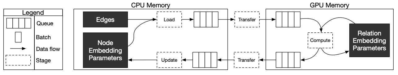
Marius follows a 5-staged pipeline architecture, 4 of which are responsible for data movement and the other is for model computation and in-GPU parameter updates. The pipeline field has options for setting thread counts for each of these stages. staleness_bound sets the maximum number of minibatches that can be present in the pipeline at any time. It implies that after a set of node embedding updates, at most of 16 mini-batches use stale node embeddings.

Partition Buffer

One of the storage backends supported for node embeddings is the PARTITION_BUFFER mode, where the nodes are bucketed into p partitions and every edge falls into one of the p^2 buckets. When pre-processed in the partitioned mode, the edges are ordered in a wat that reduces the number of node-embedding bucket swaps from the buffer.

The following command pre-processes the fb15k_237 dataset into 10 partitions as required by Marius for training in PARTITION_BUFFER mode.

marius_preprocess --dataset fb15k_237 --num_partitions 10 --output_dir /home/data/datasets/fb15k_237_partitioned/

Now, we can set the storage backend for node embeddings to PARTITION_BUFFER mode

embeddings:
  type: PARTITION_BUFFER
  options:
    dtype: float
    num_partitions: 10
    buffer_capacity: 5
    prefetching: true

num_partitions should hold the same value that was earlier supplied to marius_preprocess. buffer_capacity states the maximum number of node embedding buckets that can be present in the memory at any given time. Setting prefetching enables the system to prefetch partitions asynchronously leading to reduction in IO wait times and additional memory overheads.